asynchronous motor dimensioning with sine load

[meccanicamg]

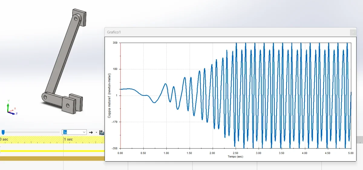
here is an approach to calculate the torque at the crank of your biella-manovella mechanism:
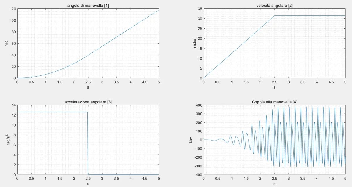
1. calculation of angular acceleration:* conversion of turns per minute to radiant per second: 1 min/60 s ≈ 31.42 rad/s
* calculation of angular acceleration: α = ω / t = 31.42 rad/s / 2.5 s ≈ 12.57 rad/s2
2. calculation of force on the piston:* determination of the force necessary to accelerate the mass: f = m
* calculation of linear acceleration of the piston: this is a more complex part because the acceleration of the piston varies during the rotation of the crank. for an approximate estimate, you can consider the maximum acceleration of the piston, which occurs when the crank is perpendicular to the biella. you can use a more detailed film analysis for a more precise calculation.
3. calculation of the tangential force on the handle:* use of the transmission ratio: the force on the piston is transmitted to the crank through the biella. the transmission ratio between the force on the piston and the tangential force on the handle depends on the geometry of the mechanism (length of the biella and the beam of the handle).
* Tangential force calculation: f_tangenziale = f_pistone * (r_manovella / l_biella)
4. calculation of the torque to the handle:* torque definition: the couple is the product of the tangential force for the crank radius.
* torque calculation: τ =
summary formulas:
* ω = 2πn / 60
* α ω / t
* f = m * a
* f_tangenziale = f_pistone * (r_manovella / l_biella)
* τ = f_tangenous * r_manovella

comments:
* approximations: this calculation provides an approximate estimate of the pair. for a more precise result, it is necessary to consider the complete kinematic analysis of the biella-manovella mechanism, taking into account the variation of the acceleration of the piston during the rotation of the crank.
* Other factors: Other factors such as friction, biella mass and losses in the mechanism can affect the actual torque required.

precise calculation of the acceleration of the piston in a biella-manovella mechanism requires a more in-depth analysis of the kinematics.

formulas and considerations:to determine the acceleration of the piston at every moment, it is necessary to consider the geometry of the mechanism and the angular speed of the handle.* piston position:
the position of the piston (s) in relation to the upper dead point can be expressed according to the angle of rotation of the crank (θ) and the lengths of the biella (l) and the crank (r):
(cos(θ) + √(l2 - r2sin2(θ)))

* piston speed:
derived the position compared to time, you get the piston speed:
v = ds/dt = ω * r * (sin(θ) + (r * sin(θ) * cos(θ) / √(l2 - r2sin2(θ)))

where ω is the angle speed of the crank.
* Piston acceleration:
further resulting the speed compared to the time, you get the acceleration of the piston:
a = dv/dt = ω2 * r * (cos(θ) + (r * (cos2(θ) - sin2(θ)) / √(l2 - r2sin2(θ)) + (r3 * sin2(θ) * cos(θ)) / (l2 - r2sin2(θ)))^(3/2))

comments:
* complexity of the equation: As you can see, the acceleration equation is quite complex and contains trigonometric terms.
* variation of acceleration: the acceleration of the piston varies continuously during the rotation of the crank, reaching maximum and minimum values at certain positions.
* graphs: to better display the variation of acceleration over time, it is useful to graphically represent acceleration according to the angle of rotation of the handle.

numerical calculations:
to obtain specific numerical values for your case, you can:
* Replace numerical values: insert r, l, ω and θ values into equations.
* use a spreadsheet: use a program like excel or an online spreadsheet to calculate acceleration for different values of θ.
* use a simulation software: software such as matlab or cad programs can be used to perform dynamic simulations of the mechanism and get detailed graphics of acceleration.

Further considerations:
* rotation angle: θ angle can vary from 0 to 2 radiant for a complete turn of the crank.
* measuring unit: Be sure to use consistent measuring units (for example, meters for lengths, radiant for angles and seconds for time).
* approximations: in some cases, approximations can be used to simplify calculations, but it is important to evaluate the accuracy of approximations according to the specific application.

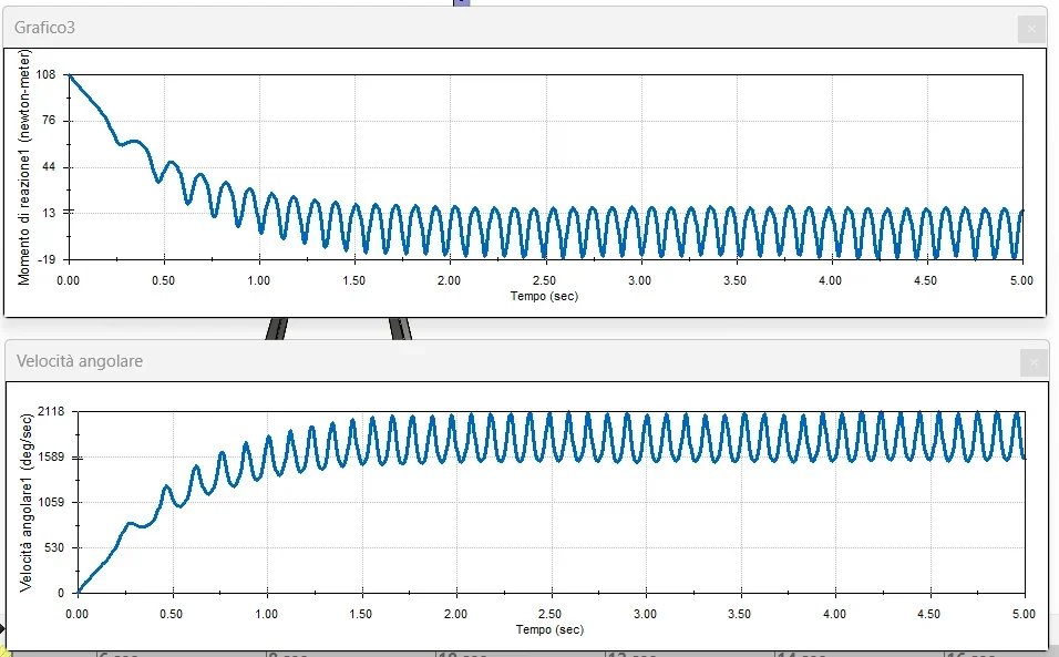
do everything with excel and you will see that you will be able to track the charts you need and then from here overlap the engine curve power/turns and torque/turns and you will assess whether it's okay or not.

Remember that depending on the starting angle you will still get different charts and torques to start different.

in all this was considered in the first unaffected approximation: friction and inertia.

built the basic calculation sheet you can enrich it with new considerations.

 

[Taipan95]

Good morning.
thanks for all your considerations and contributions. I created a small list of matlabs where I went to insert the equations of the problem (the allego).
Basically, I calculated the vertical acceleration of the piston doing the secondary derivative of its position in space, position that is parameterized on theta and phi (see figure I put at the beginning of the post). I imposed the acceleration profile and backwards I determined, numerically, the speed and angle position of the crank. also the phi angle was parameterized compared to theta, as well as by numerical way its derivatives were determined (speed and acceleration).

At this point I wrote the mass equation* acceleration = piston force, which I converted into tangential force. This, multiplied by beam of crank, gave me the pair.

plotting the graphs showing: angular acceleration of crank (1), speed (2), cumulative angle (3) [tutte in rad], and finally the driving couple (4) [in Nm].

I tried to model in solidworks a very simple system, and with the motion module I simulated it by imposing the speed profile from me wanted (from 0 to 2.5s you climb up to 300rpm, then you go constant from 2.5s to 5s).

as you can see, the two trends are identical in form and very similar in values (unless differences due to inertias, that in my accounts there are no... friction is not even in solidworks).

and here we go back to what I was trying to explain from the beginning of the post, but that because of me maybe it didn't come out well... How come, to move this system from 20kg, I need a couple in the order of 400nm? clearly it is not correct... the answer I gave me is as follows: because the system has an oscillating dynamic, if I impose an instant speed trend like in (3) I need to provide a very high torque... that trend there is not instant speed, but it should be that of the average speed around which I have the oscillations (and that was what I had posted before with the black line and the red sinusoid).

 

[meccanicamg]

Good morning.
thanks for all your considerations and contributions. I created a small list of matlabs where I went to insert the equations of the problem (the allego).
Basically, I calculated the vertical acceleration of the piston doing the secondary derivative of its position in space, position that is parameterized on theta and phi (see figure I put at the beginning of the post). I imposed the acceleration profile and backwards I determined, numerically, the speed and angle position of the crank. also the phi angle was parameterized compared to theta, as well as by numerical way its derivatives were determined (speed and acceleration).

At this point I wrote the mass equation* acceleration = piston force, which I converted into tangential force. This, multiplied by beam of crank, gave me the pair.

plotting the graphs showing: angular acceleration of crank (1), speed (2), cumulative angle (3) [tutte in rad], and finally the driving couple (4) [in Nm].

I tried to model in solidworks a very simple system, and with the motion module I simulated it by imposing the speed profile from me wanted (from 0 to 2.5s you climb up to 300rpm, then you go constant from 2.5s to 5s).

as you can see, the two trends are identical in form and very similar in values (unless differences due to inertias, that in my accounts there are no... friction is not even in solidworks).

and here we go back to what I was trying to explain from the beginning of the post, but that because of me maybe it didn't come out well... How come, to move this system from 20kg, I need a couple in the order of 400nm? clearly it is not correct... the answer I gave me is as follows: because the system has an oscillating dynamic, if I impose an instant speed trend like in (3) I need to provide a very high torque... that trend there is not instant speed, but it should be that of the average speed around which I have the oscillations (and that was what I had posted before with the black line and the red sinusoid).

the 400nm are those that correspond to the reverse of motion. At that moment, at constant speed of crank, you have a trend far from exercising the mass of the piston. the piston goes from ahead to v max to zero and sudden minus v max.
your engine or the reducer will have to deliver 400nm.

reduction ratio:
= 1400/300 = 4,7

engine 4 poles n=1400rpm
engine torque = 400/4,7 = 85nm
power die about wm = 12.5kw

since 12.5kw there is not take 11kw which is standard and we use it with the inversions above s1. Actually you could also use a 7.5kw 4p with the same logic.

If you prefer a vector engine we can use a base rpm higher 2000....3000rpm and then use a gearbox with greater and more easily supplyable ratio.

with solidworks move the mechanism and see what positions match the peaks of +/-400nm and post the image.

 

[meccanicamg]

example this attached gear motor represents a standard sew motor with coaxial reducer with a 4 pole motor and a reduction ratio that makes about the same outgoing rpm.

 

[Taipan95]

I attach you a screenshot of a very similar mechanism (unless the inertias, but for now let's ignore them) that was shown during the course I followed.

as you can see, simulated in solidworks motion, the average speed trend is exactly what you want, but instantly it swings around that value (at range between 2100 and 1500, whose average is 1800 [gradi al secondo] that are just 300 rpm) instead of being linear and accurate as the trends I posted before in matlab.

if known, the required pair is oscillating but it reaches max to 20nm (leaving the point value, focusing only on the regimen)... how is it possible? the adjustment with inverter allows me to do this?

I can't understand how it's possible that you get such a high torque discrepancy (400nm with a linear speed profile versus 20nm of an oscillator, of which the average is what interests me but not the instant value... In fact the average speed profile is exactly like the one I wanted, it puts us about 2s to get to regime and from there goes... I accept that there are oscillations instantly, it is the average in the time that I care about).

and this justifies the fact that the asynchronous motor piloted with inveter, of this application realized in reality, is plaster to 1kw of power that is well different from the 12kw that we find with the "manual" accounts.